Frustrated Phase Separation
A large variety of systems with competing short and long range interactions self-organizes in domain patterns as reviewed by Seul and Andelman. Examples range from magnetic systems (left figure A) to organic systems (left figure B).
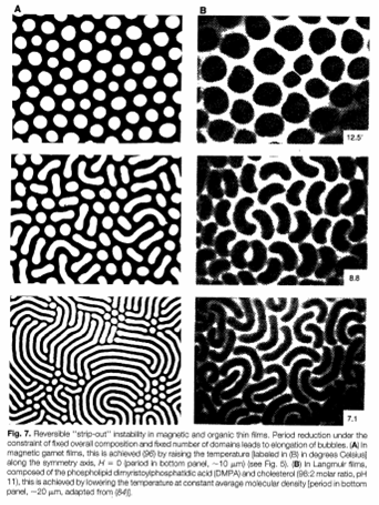
Fig. 1: Frustrated phase separation in different classical systems (From Seul and Andelman).
Inhomogeneous states display a simple set of predominant morphologies like circular droplets and stripes in two-dimensional (2D) systems, and layers, cylindrical rods and spherical droplets in three-dimensional (3D) systems. This tendency for a common behavior across different systems calls for simple models which neglect the specific details of each system and capture the general properties.
The same phenomenology has been reported in strongly correlated system as discussed in this review (see also the presentation in the attachments below).
In strongly correlated electronic systems, when the kinetic energy is suppressed by the strong Coulomb interaction, one often encounters a tendency towards phase separation. This manifest by anomalies in the electronic contribution to the free energy density. Two kind of anomalies appear often in strongly correlated systems.
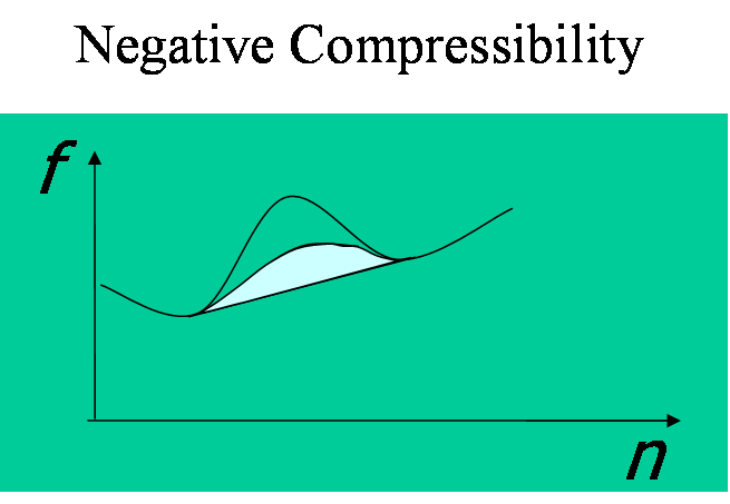
Fig. 2: Free energy as a function of the global density. The straight line is the Maxwell construction whereas the turquoise region represents the extra cost due to frustration.

Fig. 3: Idem for the case of a cusp singularity anomaly in the free energy.
The first situation is determined by a negative compressibility region i.e. a region of density n where the free energy f has negative curvature, as shown on the left green panel. A notorious example is the uniform electron gas (EG) at low density but this feature appears in several other systems from solid state to neutron star matter. The other possibility is that the inverse electronic compressibility has a point with a Dirac-delta-like negative divergence at some density. This happens when the free energies of two states which are separated by a barrier, cross each other leading to a cusp singularity (right green panel). An example is also provided by the EG. Indeed numerical simulations show that the Wigner crystal and the uniform phases free energy cross at some density.
In the absence of Coulomb repulsion phase separation is governed by the tangent or Maxwell construction (straight line in the green panels). Our fluid separates in two macroscopic regions with different densities in blue and light blue in the next panels:
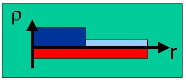
Fig. 4: Charge profile for macroscopic phase separation
If our fluid is made of electrons we have to consider also a rigid background which keeps charge neutrality (in read). Then the long range Coulomb interaction forbids macroscopic phase separation since the electrostatic cost of the above configuration grows faster than the volume. The system separates in small regions so as to gain some of the phase separation energy gain keeping the system neutral on large length scales at the cost of paying some surface energy. The turquoise region in the free energy panels represent the extra free energy cost due to Coulomb and surface energy. The following panel shows schematically the charge profile:
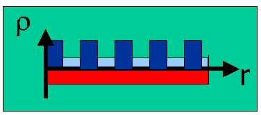
Fig. 5:Charge profile for mesoscopic phase separation.
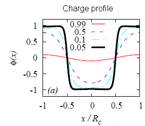
Fig. 6: Charge profile evolution for Coulomb frustrated phase separation in the case of a negative compressibility anomaly.
This charge profile corresponds to a case in which Coulomb frustration is small and inhomogeneities have a charge density which does not differ much from the one in macroscopic phase separation. In the case of a negative compressibility region for strong frustration only uniform phases are allowed. As the Coulomb frustration is reduced (parametrized by an effective charge Q) at some point the system becomes unstable to a sinusoidal charge modulation as shown by the read line in the picture. Reducing even more the frustration Q the profile gradually becomes anharmonic with sharp interfaces. The figure shows the evolution of the charge profile from strong frustration (red) to weak frustration (black). As the frustration is reduced the periodicity of the modulation grows becoming of the order of the system size when the frustration tends to zero. Thus the system can smoothly go from a sinusoidal charge density wave to macroscopic phase separation (read our article).
In the case of a cusp sigularity the situation is dramaticaly different. In two dimensions, as shown by Jamei, Kivelson, and Spivak , no mater how strong is the frustration there is always a range of densities where inhomogneneous phases appear.The following picture compares the phase diagrams in the two universality classes.
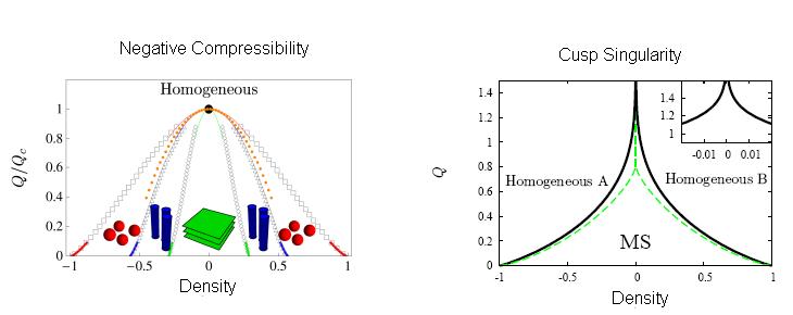
Fig. 7: Phase diagrams for the two universality classes discussed. On the left we show the case of the negative compressibility anomaly in three dimensions. We also show the topological transitions. On the right we show the phase diagram for the cusp singularity anomaly restricted to stripes in two dimensions (full line) and layers in three dimensions (dashed green line). The inset shows an enlargement of the two dimensional case displaying a logarithmic singularity.
As in classical systems inhomogeneities have different geometries depending mainly on the volume fraction. The different geometries are schematized in the negative compressibility phase diagram. Similar geometries will appear in the cusp singularity case away from the central region.
In the cusp singularity universality class for large frustration the electronic compressibility is negative and very large at the density of the cusp. In this case the model of a rigid background has to be put into question. If the background compressibility is finite the system becomes thermodynamically unstable leading to a volume collapse transition as a function of pressure. In this case we have elastically frustrated phase separation. We have discuss the thermodynamic of volume collapse transitions here and in the article below.
Another interesting issue is how phase separation occurs when the solid has a layered structure or is a two dimensional solid. We have recently discussed this case, finding the fascinating phase diagram shown in the figure below.

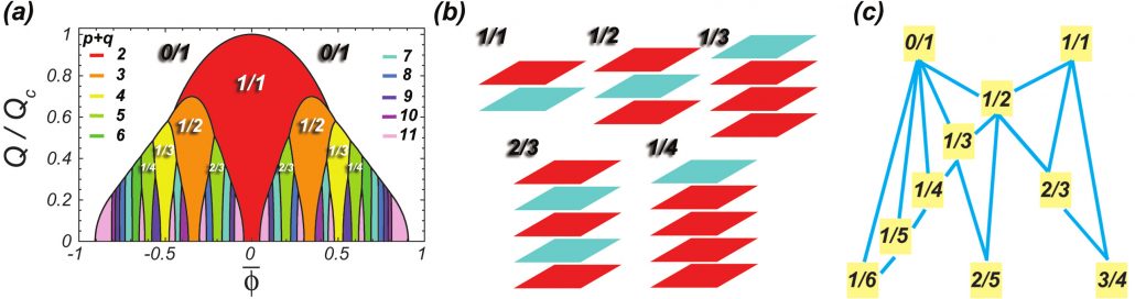
Fig. 8. (a) Phase diagram for layered frustrated phase separation in the Q (frustration) and fi (density) plane. The system phase separates in high and low density layers thus forming spontaneous heterostructures. p+q is the periodicity moving perpendicular to the layers. As Q decreases, Arnold tongues with larger periodicity appear at the expenses of the lower periodicity tongues acquiring a funnel shape ending in one point. (b) Sketch of the lowest period electronic heterostructures. The phases follow a modified Farey tree construction. Each fraction p/q is generated by its ancestors pa /qa and pb /qb as p/q = (pa + pb )/(qa + qb )
To learn more you can read this review, this shorter but more recent review, our article in Phys. Rev. Lett. or check our recent publications in the subject. Less recent publications are found below.
People: Claudio Castellani, Carlo Di Castro, Carmine Ortix, José Lorenzana.
Reference material
- Thermodynamics of volume-collapse transitions in cerium and related compounds
- Mesoscopic frustrated phase separation in electronic systems
- Presentation on Frustrated Phase Separation
- Coulomb-Frustrated Phase Separation Phase Diagram in Systems with Short-Range Negative Compressibility
- Phase separation frustrated by the long-range Coulomb interaction. I. Theory
- Phase separation frustrated by the long-range Coulomb interaction. II. Applications
- Frustrated phase separation in two-dimensional charged systems
- Screening effects in Coulomb-frustrated phase separation
- Self-organized electronic superlattices in layered materials
